Example 3: How to plot recognition performance

After the 2nd example, we get the recognition performance. This example shows how to use the build-in functions to plot recognition performance.

You can find the related code in demo/plot_performance.py or demo/plot_performance.ipynb.

In the 2nd example, we stored the results in res/benchmarkdataset_res.mat. Firstly, we need to reload these results.

from SSVEPAnalysisToolbox.utils.io import loaddata
data_file = 'res/benchmarkdataset_res.mat'
data = loaddata(data_file, 'mat')
acc_store = data["acc_store"]
itr_store = data["itr_store"]
train_time = data["train_time"]
test_time = data["test_time"]
tw_seq = data["tw_seq"]
method_ID = data["method_ID"]
method_ID = [name.strip() for name in method_ID]

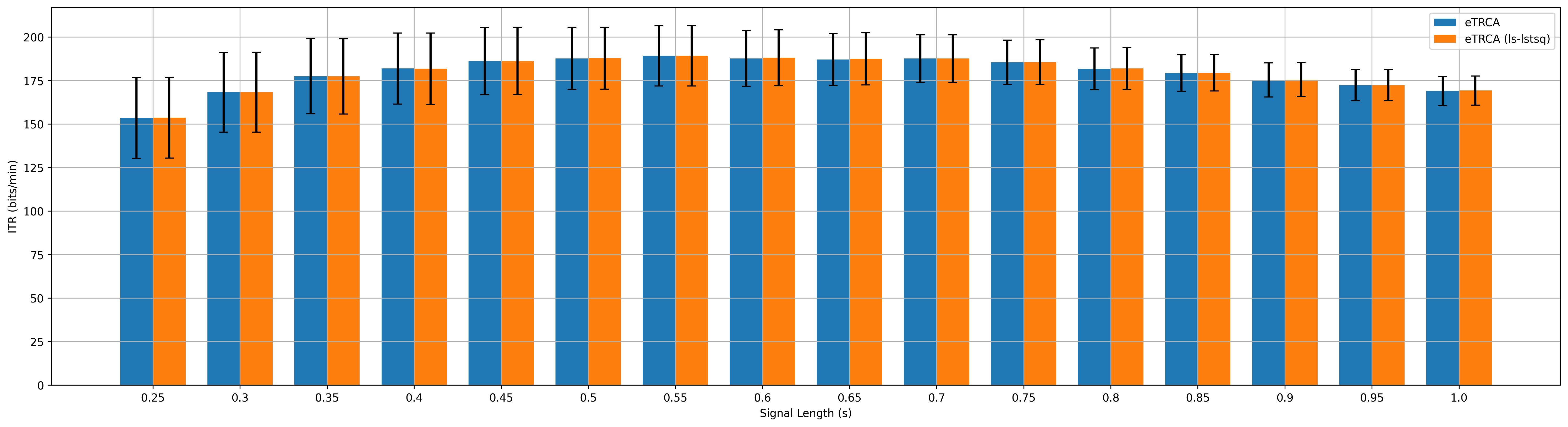
Then, we can use the build-in function to plot the recognition accuracy and ITR by using bar charts, and save the corresponding figures.

from SSVEPAnalysisToolbox.evaluator import bar_plot_with_errorbar
sub_title = 'benchmark'

fig, _ = bar_plot_with_errorbar(acc_store,
                                x_label = 'Signal Length (s)',
                                y_label = 'Acc',
                                x_ticks = tw_seq,
                                legend = method_ID,
                                errorbar_type = '95ci',
                                grid = True,
                                ylim = [0, 1],
                                figsize=[6.4*3, 4.8])
fig.savefig('res/{:s}_acc_bar.jpg'.format(sub_title), bbox_inches='tight', dpi=300)

fig, _ = bar_plot_with_errorbar(itr_store,
                                x_label = 'Signal Length (s)',
                                y_label = 'ITR (bits/min)',
                                x_ticks = tw_seq,
                                legend = method_ID,
                                errorbar_type = '95ci',
                                grid = True,
                                figsize=[6.4*3, 4.8])
fig.savefig('res/{:s}_itr_bar.jpg'.format(sub_title), bbox_inches='tight', dpi=300)

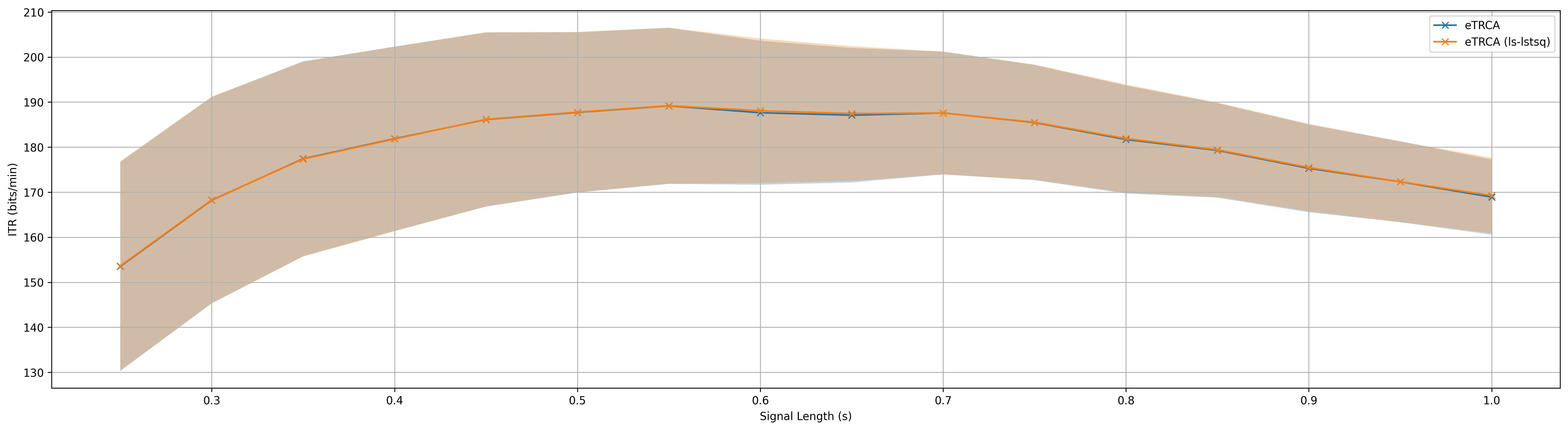
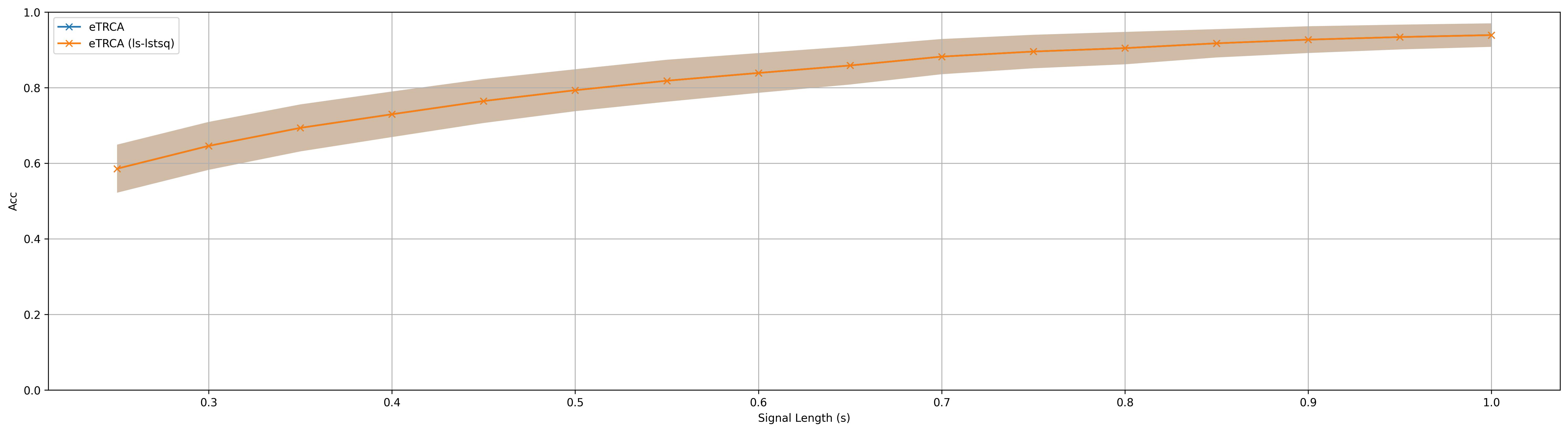
We also can plot the recognition accuracy and ITR by using the shadow lines, and save the corresponding figures.

from SSVEPAnalysisToolbox.evaluator import shadowline_plot
fig, _ = shadowline_plot(tw_seq,
                        acc_store,
                        'x-',
                        x_label = 'Signal Length (s)',
                        y_label = 'Acc',
                        legend = method_ID,
                        errorbar_type = '95ci',
                        grid = True,
                        ylim = [0, 1],
                        figsize=[6.4*3, 4.8])
fig.savefig('res/{:s}_acc_shadowline.jpg'.format(sub_title), bbox_inches='tight', dpi=300)

fig, _ = shadowline_plot(tw_seq,
                        itr_store,
                        'x-',
                        x_label = 'Signal Length (s)',
                        y_label = 'ITR (bits/min)',
                        legend = method_ID,
                        errorbar_type = '95ci',
                        grid = True,
                        figsize=[6.4*3, 4.8])
fig.savefig('res/{:s}_itr_shadowline.jpg'.format(sub_title), bbox_inches='tight', dpi=300)